Working with SimSpin FITS files

SimSpin can generate astronomy standard FITS files through the build_datacube and write_simspin_FITS functions. In this example, we take you through how to work with these files to reproduce the saved images or cubes.

For this walkthrough, we will be using a number of FITS files:

A spectral datacube FITS
A kinematic datacube FITS (made using the same configuration as the spectral cube above)
A sf gas datacube FITS

In each example, we will provide a quick description of how the file has been made and then demonstrate a way of interacting with the images and cubes.

Spectral FITS Kinematic FITS Gas FITS

Spectral FITS files

Let’s use another example file from the SimSpin package to build a spectral datacube and save to FITS. This time, we’ll use an example file from the hydrodynamical simulation EAGLE.

# Load a model...
simulation_file = system.file("extdata", "SimSpin_example_EAGLE.hdf5", package = "SimSpin")
# ... use to build a SimSpin file. 
simspin_eagle  = make_simspin_file(filename = simulation_file,
                                   template = "EMILES",
                                   write_to_file = FALSE)

# Building a datacube with default spectral parameters 
cube   = build_datacube(simspin_file = simspin_eagle,
                        telescope = telescope(),
                        observing_strategy = observing_strategy(),
                        method = "spectral",
                        write_fits = T, 
                        output_location = "SimSpin_spectral_example_EAGLE.FITS",  
                        object_name = "SimSpin_example_EAGLE",
                        telescope_name = "SimSpin",
                        observer_name = "Anonymous",
                        split_save = F)

Once the file has been built, using R we use the Rfits package to inspect the extensions in the file.

There are many other tools for inspecting FITS files written in other languages, such as the FITSio package for Python users. We continue with R here so that we can take advantage of the plotting functions available within the SimSpin package, but note that the same processes can be followed with an alternative tool.

library(Rfits)
cube = Rfits_read_all("SimSpin_spectral_example_EAGLE.FITS")
summary(cube)

#          Length  Class        Mode
#                9 Rfits_header list
# DATA     1731600 Rfits_cube   list
# OB_TABLE       3 Rfits_table  list
# RAW_FLUX     900 Rfits_image  list
# RAW_VEL      900 Rfits_image  list
# RAW_DISP     900 Rfits_image  list
# RAW_AGE      900 Rfits_image  list
# RAW_Z        900 Rfits_image  list
# NPART        900 Rfits_image  list

Here, the second extension contains the spectral datacube of interest. The object is an Rfits_cube of length 1731600 (i.e. 30 x 30 spatial bins x 1924 wavelength bins). A greater description of the elements in each of these HDU extensions can be found below.

EXT (HDU)	Name	Description
1		Header containing general information relating to the individual galaxy observed, the code version run, and placeholder values to maintain typical FITS layout.
2	DATA	The spectral cube with axes x, y, v_los. Each z-axis bin corresponds to a given wavelength, given by the axis labels. Values within each bin correspond to the amount of r-band flux at a given x-y projected location at that wavelength.
3	OB_TABLE	A table that contains all of the SimSpin run information such that a specific data cube can be recreated. Contains three columns (Name, Value, Units).
4	RAW_FLUX	An image of the raw particle r-band flux in CGS.
5	RAW_VEL	An image of the raw particle LOS velocities in units of km/s.
6	RAW_DISP	An image of the raw particle LOS velocity dispersions in units of km/s.
7	RAW_AGE	An image of the raw particle stellar ages in units of Gyr.
8	RAW_Z	An image of the raw particle metallicities in units of Z_sol.
9	NPART	An image of the raw number of particles per pixel.

To explore the spectra in the data element of this cube, we simply reference the imDat array contained in the Rfits cube list within the environment.

dim(cube$DATA$imDat)
# [1]   30   30 1924

flux_image = array(dim = c(30,30))
# Collapsing the cube to make a flux image
for (x in 1:dim(cube$DATA$imDat)[1]){
    for (y in 1:dim(cube$DATA$imDat)[2]){
        flux_image[x,y] = sum(cube$DATA$imDat[x,y,])
    }
}

plot_flux(flux_image, labN=4, units = "DATA summed image, total flux CGS") # made from flattening the spectral cube
plot_flux(cube$RAW_FLUX$imDat, labN=4, units = "RAW_FLUX image, g-band flux CGS") # the RAW_FLUX image contained in HDU 4

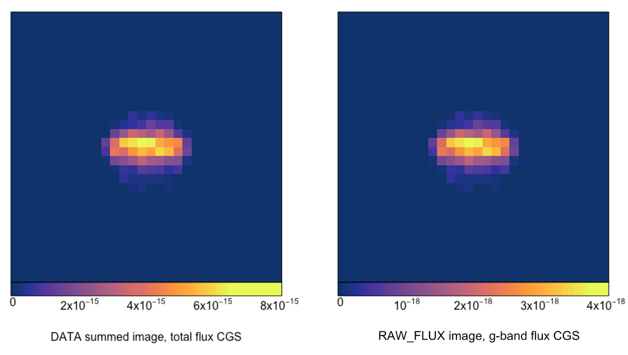
The fluxes are different in these two images. This is because the RAW_FLUX image is the sum of the flux through an g-band SDSS filter response, while the summed flux from the DATA cube is all the flux across the range of bands visible to our telescope. Despite the normalisation, the relative distribution of the flux in the two images is identicle.

We can also examine a single spectrum along one spaxel. This can be done by plotting the wavelength axis with respect to the flux at that spaxel. First, we must access the wavelength information using the observation details within the OB_TABLE at HDU 3. The information in this table is stored as strings, and so we must convert the values to numeric floats before proceeding. This is done using the stringr package, which can be downloaded directly from CRAN with the command install.packages("stringr").

We use the magicaxis package to make these plots, which can also be downloaded directly from CRAN with the command install.packages("magicaxis").

cube$OB_TABLE
#               Name               Value     Units
# 1:        ang_size             1.00032     num: scale at given distance in kpc/arcsec
# 2:  aperture_shape            circular     str: shape of aperture
# 3:   aperture_size             15.0048     num: field of view diameter width in kpc
# 4:            date 2023-03-30 16:25:01     str: date and time of mock observation
# 5:             fov                  15     num: field of view diameter in arcsec
# 6:          filter              g_SDSS     str: filter name
# 7:         inc_deg                  70     num: projected inclination of object in degrees about the horizontal axis
# 8:         inc_rad             1.22173     num: projected inclination of object in radians about the horizontal axis
# 9:       twist_deg                   0     num: projected inclination of object in degrees about the vertical axis
#10:       twist_rad                   0     num: projected inclination of object in radians about the vertical axis
#11:        lsf_fwhm                2.65     num: line-spread function of telescope given as full-width half-maximum in Angstrom
#12:        lum_dist              227.48     num: distance to object in Mpc
#13:          method            spectral     str: name of observing method employed
#14:          origin    SimSpin_v2.4.5.5     str: version of SimSpin used for observing
#15:    pointing_kpc                 0,0     num: x-y position of field of view centre relative to object centre in units of kpc
#16:    pointing_deg                 0,0     num: x-y position of field of view centre relative to object centre in units of deg
#17:        psf_fwhm                   0     num: the full-width half-maximum of the point spread function kernel in arcsec
#18:            sbin                  30     num: the number of spatial pixels across the diameter of the field of view
#19:        sbin_seq      -7.5024,7.5024     num: the min and max spatial bin centres in kpc
#20:       sbin_size             0.50016     num: the size of each pixel in kpc
#21:     spatial_res                 0.5     num: the size of each pixel in arcsec
#22: signal_to_noise                None     num: the signal-to-noise ratio for observed spectrum
#23:        wave_bin                1924     num: the number of wavelength bins for a given telescope
#24:     wave_centre                4700     num: the central wavelength for a given telescope in Angstrom
#25:        wave_res                1.04     num: the width of each wavelength bin in Angstrom
#26:        wave_seq        3700,5699.92     num: the min and max wavelength bin centres in Angstrom
#27:      wave_edges     3699.48,5700.44     num: the wavelength bin edges in Angstrom
#28:       vbin_size             66.3371     num: the size of each velocity bin in km/s
#29:      vbin_error             71.7812     num: the velocity uncertainty given the telescope LSF in km/s
#30:               z                0.05     num: the redshift distance of the object observed
#31:        LSF_conv                TRUE     bool: has line spread function convolution been applied?
#32:       lsf_sigma            0.113041     num: line-spread function of telescope given as a sigma width in Angstrom
#               Name               Value     Units

wavelength_range = as.numeric(stringr::str_split(string = cube$OB_TABLE$Value[26], pattern = ",")[[1]]) 
wavelength_seq   = seq(wavelength_range[1], wavelength_range[2], by = as.numeric(cube$OB_TABLE$Value[25])) 

# examining the central spaxel of the output spectral cube:
magicaxis::magplot(wavelength_seq, cube$DATA[["imDat"]][15,15,], type="l", col = "purple", lwd =2, xlab = "Wavelength, Angstroms", ylab = "Luminosity, CGS")

Kinematic FITS files

In this example, we will build a kinematic cube and plot the observed line-of-sight velocity distribution (LOSVD) using the information contained within the extension header, rather than the associated observation OB_TABLE.

First, let’s build another cube.

# Building a kinematic datacube with default parameters using the same SimSpin file
cube   = build_datacube(simspin_file = simspin_eagle,
                        telescope = telescope(),
                        observing_strategy = observing_strategy(),
                        method = "velocity",
                        write_fits = T, 
                        output_location = "SimSpin_velocity_example_EAGLE.FITS",  
                        object_name = "SimSpin_example_EAGLE",
                        telescope_name = "SimSpin",
                        observer_name = "Anonymous",
                        split_save = F)

library(Rfits)
cube = Rfits_read_all("SimSpin_velocity_example_EAGLE.FITS")
summary(cube)

#          Length Class        Mode
#              9  Rfits_header list
# DATA     27000  Rfits_cube   list
# OB_TABLE     3  Rfits_table  list
# OBS_FLUX   900  Rfits_image  list
# OBS_VEL    900  Rfits_image  list
# OBS_DISP   900  Rfits_image  list
# OBS_H3     900  Rfits_image  list
# OBS_H4     900  Rfits_image  list
# RESIDUAL   900  Rfits_image  list
# RAW_FLUX   900  Rfits_image  list
# RAW_VEL    900  Rfits_image  list
# RAW_DISP   900  Rfits_image  list
# RAW_AGE    900  Rfits_image  list
# RAW_Z      900  Rfits_image  list
# NPART      900  Rfits_image  list

Because we have built a velocity cube this time, the output list has several additional images output, the observed_images produced by the code fitting the observed LOSVD, including OBS_FLUX, OBS_VEL, OBS_DISP, OBS_H3 and OBS_H4.

In this case, the DATA Rfits cube is smaller due to the reduced number of velocity channels (in comparison to the wavelength range of a given telescope) i.e. 30 x 30 spatial planes by 30 velocity planes = 27000.

Reading in this velocity cube, we can examine the axes of the cube in order to plot the LOSVD using the keyvalues within the Rfits cube.

velocity_cube = cube[["DATA"]]$imDat # The kinematic data cube is stored in the first HDU 
                                     #  (can also be accessed cube$imDat).

header = cube[["DATA"]]$keyvalues    # The keyvalues header of the file gives everything 
                                     #  you need to assign values to the cube axes.

spatial_range = header$CRVAL1 + (seq(header$CRPIX1, header$NAXIS1)*header$CDELT1)
                                     # We use the first or second inputs to the axDat to describe
                                     #  the spatial axes of the cube. As the aperture is square, 
                                     #  the first and second inputs give the same answer.

velocity_range = header$CRVAL3 + (seq(header$CRPIX3, header$NAXIS3)*header$CDELT3)
                                     # Because the velocity is the third axis of the cube, we use 
                                     #  the third element in the axDat element to define the velocity
                                     #  range. 

The elements of the keyvalues header are defined in the table below:

`CRPIX`	The pixel index at which values are defined. Default (1,1,1).
`CRVAL`	The value associated with the `CRPIX` pixel.
`CDELT`	The difference in value between each pixel.
`NAXIS`	The dimensions of the cube (number of pixels along each axis).
`CTYPE`	The name that defines each dimension of the cube.
`CUNIT`	The units for each dimension of the cube.

We can then use these axes to plot and fit the observed LOSVD.

# Defining a function to fit the observed line-of-sight velocity distribution:
losvd_fit = function(par, x, losvd){
  
  vel = par[1]
  sig = par[2]
  h3  = par[3]
  h4  = par[4]
  
  w = (x - vel)/sig
  H3 = (1/sqrt(6))  * (((2*sqrt(2))* w^3) - ((3*sqrt(2)) * w))
  H4 = (1/sqrt(24)) * ((4* w^4) - (12 * w^2) + 3)
  
  measured_vlos = (exp(-0.5*(w^2)) * (1 + (h3*H3) + (h4*H4)))
  return=sum((measured_vlos-losvd)^2)
}

# Then, a function to generate this function given a range of supplied 
#  velocities and the parameters of the Gauss-Hermite fit. 

losvd = function(x, vel, sig, h3, h4){
  w = (x - vel)/sig
  H3 = (1/sqrt(6))  * (((2*sqrt(2))* w^3) - ((3*sqrt(2)) * w))
  H4 = (1/sqrt(24)) * ((4* w^4) - (12 * w^2) + 3)
  
  measured_vlos = (exp(-0.5*(w^2)) * (1 + (h3*H3) + (h4*H4)))
  return(measured_vlos)
}

# Fitting the LOSVD at the central pixel of the observed velocity cube:
losvd_obs = stats::optim(par   = c(0,100,0,0),
                         fn    = losvd_fit,
                         x     = velocity_range,
                         losvd = (velocity_cube[15,15,]/(max(velocity_cube[15,15,], na.rm=T))),
                         method="BFGS")$par

# Plotting the observed LOSVD and given fit:
library(magicaxis)
magplot(velocity_range, velocity_cube[15,15,]/(max(velocity_cube[15,15,])), 
        xlab = expression("Velocity"[LOS]*", km/s"), type="p", pch=16)
lines(velocity_range, 
      losvd(velocity_range, 
            vel = losvd_obs[1], 
            sig = losvd_obs[2], 
            h3 = losvd_obs[3], 
            h4 = losvd_obs[4]),
      col = "purple", lwd = 2)

The returned LOSVD parameters give us a line-of-sight velocity of 52 km/s at the galaxy centre, and a dispersion of 148 km/s. The same approach is followed for every pixel in the cube, using the flux-weighted LOS velocity and dispersions as priors on the losvd_fit function within the SimSpin code.

Gas FITS files

Finally, we will demonstrate the output kinematic cube produced through mock observations of the gas component of the galaxy model.

Let’s build our final cube.

# Building a datacube using the gas method
cube   = build_datacube(simspin_file = simspin_eagle,
                        telescope = telescope(),
                        observing_strategy = observing_strategy(),
                        method = "gas",
                        write_fits = T, 
                        output_location = "SimSpin_gas_example_EAGLE.FITS",  
                        object_name = "SimSpin_example_EAGLE",
                        telescope_name = "SimSpin",
                        observer_name = "Anonymous",
                        split_save = F)

In this example, we examine all of the gas particles in the model. If specifying method = "sf gas", we could limit this to only gas that meets a given star formation threshold, such as having met the equation of state criterion of that simulation, or a given temperature cut.

library(Rfits)
cube = Rfits_read_all("SimSpin_gas_example_EAGLE.FITS")
summary(cube)

#          Length Class        Mode
#              9  Rfits_header list
# DATA     14400  Rfits_cube   list
# OB_TABLE     3  Rfits_table  list
# OBS_MASS   900  Rfits_image  list
# OBS_VEL    900  Rfits_image  list
# OBS_DISP   900  Rfits_image  list
# OBS_H3     900  Rfits_image  list
# OBS_H4     900  Rfits_image  list
# RESIDUAL   900  Rfits_image  list
# RAW_MASS   900  Rfits_image  list
# RAW_VEL    900  Rfits_image  list
# RAW_DISP   900  Rfits_image  list
# RAW_Z      900  Rfits_image  list
# RAW_OH     900  Rfits_image  list
# RAW_SFR    900  Rfits_image  list
# NPART      900  Rfits_image  list

These gas cubes are very similar in structure to the kinematic cubes produced in the example above. Each DATA cube contains spatial information in the x-y plane (30 x 30) and velocity information as we proceed depth-wise (i.e. 30 x 30 x 16 = 14400). Following the methodology from the kinematic example above, you could produce a very similar fitted LOSVD for a single pixel.

Instead, let’s examine a few of the maps included within the observation. There are several new HDU extensions, in comparison to the stellar kinematic cubes.

# Masking out pixels conatining no gas particles. 
mask = cube$NPART$imDat
mask[mask == 0] = NA

# Using the `fig` and `new` parameters, we can add multiple 
#  panels to a single plot.

# Plotting the observed gas mass per pixel
plot_mass(cube$OBS_MASS$imDat*mask, 
          fig = c(0,0.25,0,1), 
          labN = 1, titleshift = -8)

# Plotting the mean gas metallicity per pixel
plot_metallicity(cube$RAW_Z$imDat*mask, 
                 fig = c(0.25,0.5,0,1), 
                 labN = 1, titleshift = -8, new=T)

# Plotting the mean, instantaneous star formation rate (SFR) mass per pixel
plot_SFR(cube$RAW_SFR$imDat*mask, 
          fig = c(0.5,0.75,0,1), 
          labN = 1, titleshift = -8, new=T)

# Plotting the mean chemical abundance - oxygen over hydrogen - per pixel
plot_OH(cube$RAW_OH$imDat*mask, 
        fig = c(0.75,1,0,1), 
        labN = 1, titleshift = -8, new=T)

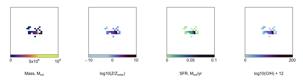
There is a relatively sparse distribution of gas in comparision the stellar distribution, but this is simply due to the construction of the example files contained within the SimSpin package.

We can see that there is a number of raw images to summarise the properties of the underlying gas, including the raw particle kinematics, the metallicity, the instantaneous star-formation rate and the chemical abundance given by log10(O/H) + 12. These raw images will not include the effects of seeing in their output.

Having demonstrated how to interact with a variety of different FITS files and their default outputs, we invite you to try these examples for yourself.

If you have any questions about anything discussed above, or suggestions about how to improve the code or example, please raise an issue using GitHub using the button below. Else, happy observing!

Raise an issue