Fitting stellar kinematics using pPXF
In order to produce observables from spectral data cubes, we must first process the outputs using external software. In this example, we demonstrate how an IFS cube produced using SimSpin can be fit using the industry standard, pPXF.
When making an observation using an IFU, the observed spectra at each pixel must be fit to determine the observed kinematics. Most commonly, the penalised pixel fitting software, pPXF (Cappellari & Emsellem 2004) is used by IFU surveys to produce observable kinematics.
The spectral cubes built by SimSpin are directly compatible with this software. In the example below, we demonstrate how to run a spectral SimSpin cube through pPXF in order to measure the observed line-of-sight velocity distribution. As pPXF is a Python code, we will present some python functions for reading and fitting the SimSpin FITS files produced in the previous example Working with FITS.
We break this down into a series of steps:
Installing pPXF
First, let’s ensure we have pPXF installed. This can be done simply using the command:
pip install ppxf
This should also download the necessary dependencies. To check that this has installed correctly, run:
pip show ppxf

# Name: ppxf
# Version: 8.1.0
# Summary: pPXF: Full Spectrum and SED Fitting of Galactic and Stellar Spectra
# Home-page: https://purl.org/cappellari/software
# Author: Michele Cappellari
# Author-email: michele.cappellari@physics.ox.ac.uk
# License: Other/Proprietary License
# Location: /path/to/lib/python3.9/site-packages
# Requires: astropy, matplotlib, numpy, scipy
# Required-by:
This tells us that we have the software installed and the location at which the package has been installed. Once this is successful, we can begin the process of fitting a SimSpin observation. We will use a similar proceadure to generate the spectral FITS as in the previous example. That was done using the R code below:
# Load a model...
simulation_file = system.file("extdata", "SimSpin_example_EAGLE.hdf5", package = "SimSpin")
# ... use to build a SimSpin file.
simspin_eagle  = make_simspin_file(filename = simulation_file,
                                   template = "EMILES",
                                   write_to_file = FALSE)

# Building a datacube with a few modified spectral parameters
cube   = build_datacube(simspin_file = simspin_eagle,
                        telescope = telescope(lsf_fwhm=3.6,
                                              fov=10,
                                              aperture_shape="hexagonal",
                                              signal_to_noise = 30),
                        observing_strategy = observing_strategy(),
                        method = "spectral",
                        write_fits = T,
                        output_location = "SimSpin_spectral_example_EAGLE.FITS",
                        object_name = "SimSpin_example_EAGLE",
                        telescope_name = "SimSpin",
                        observer_name = "Anonymous",
                        split_save = F)
The SimSpin_spectral_example_EAGLE.FITS file produced by this function will be used in the fitting procedure. For ease running as a function with parameters, we have organised the pPXF fitting code with ArgParse, such that the arguments for each pPXF fit can be passed in from the command line. The full code for this automation can be found here on GitHub, but we take you through each of the steps below.
Let’s begin by importing the necessary packages and functions:
# Importing the maths and astronomy packages required for performing pPXF fits.

import numpy as np
from astropy.io import fits
from astropy.coordinates import Angle
import matplotlib.pyplot as plt
from scipy.stats import scoreatpercentile
from scipy import ndimage,signal
import glob
import os
import sys

from matplotlib.ticker import MultipleLocator
from mpl_toolkits.axes_grid1 import make_axes_locatable
import matplotlib.ticker as ticker

from ppxf.ppxf import ppxf, rebin
import ppxf.ppxf_util as util
from ppxf import miles_util as lib
Once these steps are done, we are ready to start fitting with pPXF!
Reading in the observation
The methodology behind pPXF is that a series of template spectra are broadened by a LOSVD and iteratively fit to the observed spectrum to find the best fitting combination of parameters. There are several preparatory steps before we begin this process, however. Let’s begin by declaring the paths and variables required for running the fit. We would like to fit for V, \(\sigma\), \(h_3\) and \(h_4\) (i.e. 4 moments of the LOSVD).
#### INPUT VARIABLES ####
c = 299792.458 # speed of light in km/s
template_loc = "path/to/lib/python3.9/site-packages/ppxf/miles_models/Eun1.30*.fits" # path to the template spectra used for pPXF fitting
FWHM_temp = 2.51 # Angstrom (resolution of the template EMILES spectra used for fitting)
file_input = "SimSpin_spectral_example_EAGLE.FITS" # spectral cube generated using SimSpin
n_mom = 4 # number of LOSVD moments to compute
ppxf_output = "path/to/ppxf_output"
plot_fit = True

# Make a new pPXF fit folder at the location of ppxf_out_root for fitting plots
try:
  os.makedirs(f"{ppxf_output}/pPXF_fits", exist_ok=True)
except OSError as error:
  print("Invalid path name for output pPXF files. \n")
  sys.exit()

############################
First, we will bring all of the observed spectra back to the rest-frame. This is done because our pPXF fitting template spectra are at rest-frame. This requires us to know the observational redshift of the spectra (as given in the OB_TABLE under z). In this example, the simulated galaxy has been put at z = 0.05, so we use this to de-shift the observed spectrum.
It is also necessary to convolve the templates with a Gaussian such that the line-spread-functions (LSF) of the mock observation and the pPXF fitting templates match. As the cubes have been built from SimSpin template spectra themselves which have an underlying LSF intrinsically (before the addition of the observing telescope LSF), we need to take this into account. In this case, we used EMILES as our templates from which the SimSpin file was built. These templates have an intrinsic LSF = 2.51 A.
#---------------------------------#
# Step 1: Read in the observation #
#---------------------------------#

z = 0.05  # observed redshift of the model galaxy
telescope_FWHM = 3.6  # as specified in the telescope function
SimSpin_template_FWHM  = 2.51 # as dictated by the spectra from which the SimSpin file was built

# If the observing telescope had a requested LSF *less* than the templates themselves, we just use the reshifted SimSpin intrinsic template LSF as the value associated with the observed spectra.
if telescope_FWHM <= SimSpin_template_FWHM:
    FWHM_gal = (SimSpin_template_FWHM * (1 + z)) # Angstroms (resolution for this "observed" template)
else:
    FWHM_gal = telescope_FWHM

hdu = fits.open(f"{file_input}")

cube     = hdu["DATA"].data    # accessing the spectral datacube within the file
head_obs = hdu["DATA"].header  #    and the associated axes labels

var      = hdu["STAT"].data*1e40 # reading in the variance cube and adjusting the units
npart    = hdu["NPART"].data  # number of particles per pixel (used to describe the level of noise per pixel).

hdu.close()

print(f"Reading spectral cube of size {cube.shape}.")

# Reshape the cube into an array
npix = cube.shape[0]
nspec = cube.shape[1] * cube.shape[2]
spectrum = cube.reshape(npix, -1) # create an array of spectra [npix, (sbin_x * sbin_y)]
npart_flat = npart.reshape(-1)
npart_flat[npart_flat == 0] = None

noise_flat = var.reshape(npix, -1)

print(f"Re-shaping into array of shape {spectrum.shape}, with {spectrum.shape[0]} wavelengths and {spectrum.shape[1]} pixels.")
print(f"Re-shaping noise into array of shape {noise_flat.shape}, with {noise_flat.shape[0]} wavelengths and {noise_flat.shape[1]} pixels.")

# Begin by pulling out the wavelength axis of the cube -------------------------------------------------------------
# These properties are necessary for logarithmically re-binning the spectra before
# fitting with pPXF.
wave_axis = head_obs['CRVAL3'] + (np.arange(0., (head_obs['NAXIS3']))*head_obs['CDELT3'])
wave_range = head_obs["CRVAL3"] + np.array([0., head_obs["CDELT3"]*(head_obs["NAXIS3"]-1)])
velscale = c * np.diff(np.log(wave_axis[-2:])) # velocity step
velscale = velscale[0]

print(f"The velocity scale of the `observed` spectrum is {velscale} km/s per pixel.")

# We also need to bring the observed spectrum back to the rest-frame ------------------------------------
if z >= 0.0:
    wave_range = wave_range / (1 + z)
    FWHM_gal = FWHM_gal / (1 + z)
    z = 0
    print(f"The wavelength range of the 'observed' galaxy (returned to rest-frame) is {wave_range} Angstrom.")
    print(f"The FWHM at this restframe is {FWHM_gal}.")

else:
    print(f"The wavelength range of the 'observed' galaxy is {wave_range} Angstrom.")
    print(f"The FWHM of the observation is {FWHM_gal}.")
With these parameters ready, we next need to read in the templates we’ll use to fit the observed spectra.
Reading in the pPXF templates
In order to fit for the observed kinematics, we use a selection of template spectra for which the line-spread function (LSF) is well catagorised and broaden our templates to match the LSF of the observation. It is assumed then, that any remaining difference between the observed spectrum through the telescope and the template spectra is due to the velocity and dispersion of the source observed.
It is important to remember that we have built our models with spectra that also have an intrinsic LSF. Hence, if the requested telescope has a lsf_fwhm value below that of the intrinsic value of the spectral templates used to build the SimSpin file, we will end up with a broader LSF than expected from the specification in telescope().
We’ve written this example to automatically account for the LSF of the spectra from which the file was built, the LSF of the telescope used to build the mock observation and the LSF of the templates being used to fit the observation. A warning is also issued by SimSpin when building a spectral cube with templates that mismatch the requested telescope LSF.
We begin by reading in the template spectra commonly used for kinematic fits contained within the pPXF source code. These are MILES models with a known LSF of 2.51A.
As we’ve made our observation with a telescope LSF\(_{FWHM}\) = 3.6, we will use this information to convolve our templates with the root square difference between the template and observed LSF.
#---------------------------------#
# Step 2: Read in the templates   #
#---------------------------------#
# Next, load the templates necessary to perform the fit with pPXF

# Using pPXF function to read in the templates located at `template_loc`, this
# function reads each template spectrum into an array sorted by age and metallicity.
# If the FWHM_gal is larger than the FWHM_temp, this function will also convolve
# the templates down to the same resolution as the observations.

print(f"The FWHM of the templates is {FWHM_temp}.")
if FWHM_gal <= FWHM_temp:
    FWHM_gal = None
    print(f"No convolution can be made. Setting FWHM_gal = None.")

# In this function, the templates are convolved with the root square difference between FWHM_gal and FWHM_temp, unless the value FWHM_gal = None
miles = lib.miles(pathname = template_loc, velscale = velscale, FWHM_gal = FWHM_gal, FWHM_tem = FWHM_temp, norm_range=[5000, 5950])

templates = miles.templates
stars_templates = templates.reshape(templates.shape[0], -1)
stars_templates /= np.median(stars_templates) # Normalizes stellar templates by a scalar

log_lam_temp = miles.ln_lam_temp # wavelength axis in log-space of the templates

# masking the templates in wavelength space such that they are only 1000A longer than the observation (reducing the computation required to perform the fit)
mask = (np.exp(log_lam_temp) > (np.min(wave_range)-500)) & (np.exp(log_lam_temp) < (np.max(wave_range)+500))
log_lam_temp = log_lam_temp[mask]
stars_templates = stars_templates[mask]

wave_range_temp =[np.exp(np.min(log_lam_temp)), np.exp(np.max(log_lam_temp))]

print(f"The wavelength range of the template spectra is {wave_range_temp} Angstrom.")
print(f"Array of templates containing shape {stars_templates.shape}.")
Now that we have our templates and observation, we can perform the fit for the observed kinematics.
Running the fit
The final step of the process is to run the fit to return the observed LOSVD. In this example, we’ll fit for four moments of the LOSVD, but a similar process is followed to fit just the observed \(V\) and \(\sigma\) through the use of moments = 2 rather than moments = 4.
#----------------------------------------#
# Step 3: Fitting the observed spectra   #
#----------------------------------------#

# Preparing the galaxy observations for input into pPXF
galaxy, log_lam_galaxy, velscale = util.log_rebin(wave_range, spectrum[:,11], velscale=velscale)
galaxy /= np.median(galaxy)

dv = (log_lam_temp[0] - log_lam_galaxy[0])*c
vel = c*np.log(1 + z)
start = [vel, 100.] # starting guess for kinematic measurements

print(f"The starting guess velocity, as according to Cappellari 2017 [V = c*log(1 + z)] is {vel} km/s.")

# Now fitting each pixel in turn and comparing to the LOS_VEL and LOS_DISP values ----------------------------------
if n_mom == 2:
    ppxf_velocity    = np.empty_like(npart_flat)
    ppxf_dispersion  = np.empty_like(npart_flat)
    ppxf_chi2        = np.empty_like(npart_flat)
else:
    ppxf_velocity    = np.empty_like(npart_flat)
    ppxf_dispersion  = np.empty_like(npart_flat)
    ppxf_h3          = np.empty_like(npart_flat)
    ppxf_h4          = np.empty_like(npart_flat)
    ppxf_chi2        = np.empty_like(npart_flat)

print(f"The 'observed' spectrum has a staring wavelength of {log_lam_galaxy[0]} Angstrom.")
print(f"The template spectrum has a staring wavelength of {log_lam_temp[0]} Angstrom.")
print(f"The difference is therefore {dv} km/s.")

for j in range(nspec):
    if npart_flat[j] > 0:
        print(f"Fitting pixel [{j}]...")
        galaxy, log_lam_galaxy, velscale = util.log_rebin(wave_range, spectrum[:,j], velscale=velscale)
        noise_rebin, log_lam_noise, velscale_2 = util.log_rebin(wave_range, 1/np.sqrt(noise_flat[:,j]), velscale=velscale)
        noise_rebin /= np.median(galaxy)
        galaxy /= np.median(galaxy)

        if n_mom == 2:
            pp = ppxf(stars_templates, galaxy, noise_rebin, velscale, start,
                      vsyst=dv, lam = np.exp(log_lam_galaxy),
                      plot=False, moments=2, degree=-1, mdegree=10,  # Set plot to False when using in batch mode. change mdegree=10 for testing
                      clean=False, regul=False)

            ppxf_velocity[j]   = pp.sol[0]
            ppxf_dispersion[j] = pp.sol[1]
            ppxf_chi2[j]       = pp.chi2

            if plot_fit:
              pp.plot()
              plt.savefig(f"{ppxf_output}/pPXF_fit/pPXF_fit_{j}.png")

        else:
            pp = ppxf(stars_templates, galaxy, noise_rebin, velscale, start,
                      vsyst=dv, lam = np.exp(log_lam_galaxy), bias = 0,
                      plot=False, moments=4, degree=-1, mdegree=10,  # Set plot to False when using in batch mode. change mdegree=10 for testing
                      clean=False, regul=False)

            ppxf_velocity[j]   = pp.sol[0]
            ppxf_dispersion[j] = pp.sol[1]
            ppxf_h3[j]         = pp.sol[2]
            ppxf_h4[j]         = pp.sol[3]
            ppxf_chi2[j]       = pp.chi2

            if plot_fit:
              pp.plot()
              plt.savefig(f"{ppxf_output}/pPXF_fit/pPXF_fit_{j}.png")


    else:
        if n_mom == 2:
            print(f"Pixel [{j}] is empty, proceading to next one...")
            ppxf_velocity[j]   = np.nan
            ppxf_dispersion[j] = np.nan
            ppxf_chi2[j]       = np.nan

        else:
            print(f"Pixel [{j}] is empty, proceading to next one...")
            ppxf_velocity[j]   = np.nan
            ppxf_dispersion[j] = np.nan
            ppxf_h3[j]         = np.nan
            ppxf_h4[j]         = np.nan
            ppxf_chi2[j]       = np.nan


fit_velocity   = ppxf_velocity.reshape([cube.shape[1], cube.shape[2]])
fit_dispersion = ppxf_dispersion.reshape([cube.shape[1], cube.shape[2]])
fit_chi2       = ppxf_chi2.reshape([cube.shape[1], cube.shape[2]])

np.save(f"{ppxf_output}/SimSpin_spectral_example_EAGLE_ppxf_velocity.npy", fit_velocity)
np.save(f"{ppxf_output}/SimSpin_spectral_example_EAGLE_ppxf_dispersion.npy", fit_dispersion)
np.save(f"{ppxf_output}/SimSpin_spectral_example_EAGLE_ppxf_chi2.npy", fit_chi2)

if n_mom == 4:

    fit_h3 = ppxf_h3.reshape([cube.shape[1], cube.shape[2]])
    fit_h4 = ppxf_h4.reshape([cube.shape[1], cube.shape[2]])
    np.save(f"{ppxf_output}/SimSpin_spectral_example_EAGLE_ppxf_h3.npy", fit_h3)
    np.save(f"{ppxf_output}/SimSpin_spectral_example_EAGLE_ppxf_h4.npy", fit_h4)
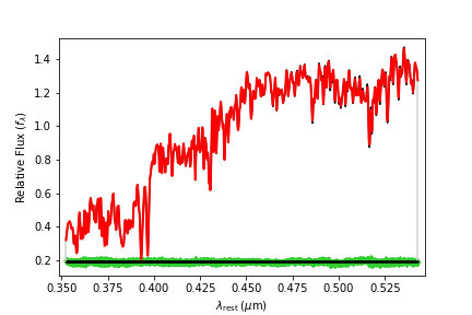
We’ve now produced a series of 2D array images where the spectrum from every pixel in our cube has been fit and the kinematic moments recorded. We can take a look at one example of the fit spectrum below:
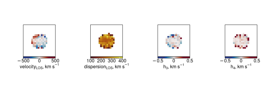
Then considering the resulting maps of the V, \(\sigma\), \(h_3\) and \(h_4\), we can use the reticulate package to read numpy arrays into R for plotting using the inbuilt SimSpin functions (or just use your favourite plotting routines in Python directly).
library(reticulate)
np = import("numpy", convert = T)
fname = "path/to/ppxf_output/SimSpin_spectral_example_EAGLE"

ppxf_example =
  list(ppxf_velocity   = t(np$load(paste0(fname, "_ppxf_velocity.npy"))),
       ppxf_dispersion = t(np$load(paste0(fname, "_ppxf_dispersion.npy"))),
       ppxf_h3  = t(np$load(paste0(fname, "_ppxf_h3.npy"))),
       ppxf_h4 = t(np$load(paste0(fname, "_ppxf_h4.npy"))),
       ppxf_chi2 = t(np$load(paste0(fname, "_ppxf_chi2.npy"))))

plot_velocity(ppxf_example$ppxf_velocity, fig = c(0,0.25,0,1), labN = 2, titleshift = -6)
plot_dispersion(ppxf_example$ppxf_dispersion, fig = c(0.25,0.5,0,1), new = T, labN = 2, titleshift = -6)
plot_h3(ppxf_example$ppxf_h3, fig = c(0.5,0.75,0,1), new = T, labN = 2, titleshift = -6)
plot_h4(ppxf_example$ppxf_h4, fig = c(0.75,1,0,1), new = T, labN = 2, titleshift = -6)
You have now completed the walk-through of fitting a small spectral SimSpin observation using pPXF.
If you have any questions about anything discussed above, or suggestions about how to improve the code or example, please raise an issue using GitHub using the button below. Else, happy observing!