Constructing your data cube

Recent Updates

With a telescope and observing_strategy, we can now make an observation of a simulated galaxy.

The output of this function will be a mock IFS data cube. The details of the observation will vary depending on the requested method, telescope and observing_strategy, but the format of the output will be consistent. In all cases, the observation can be written to a FITS file.

The following code shows the default parameters used in the build_datacube function. Calling the function without specifying any input will produce an observation with the following properties:

build_datacube(simspin_file,                     # REQUIRED input SimSpin file      
               telescope,                        # REQUIRED telescope class description
               observing_strategy,               # REQUIRED observing_strategy class description
               method = "spectral",              # "spectral", "velocity", "gas" or "sf_gas"
               verbose = F, 
               write_fits = F, output_location,  # write to a FITS file? If so, where?
               object_name = "GalaxyID_unknown", # information for FITS file headers
               telescope_name = "SimSpin",
               observer_name = "Anonymous",
               split_save = F, cores = 1,        
               mass_flag = F,                    # mass or luminosity-weighted? (if method = "velocity").
               voronoi_bin = F,                  # should we bin pixels until they meet a 
               vorbin_limit = 10)                #   minimum number of particles limit?

Input parameters Output parameters See an example See the source code

As of version 2.2.0, the method input parameter has been moved directly to the build_datacube function. For backwards compatibility, this parameter can still be specified within telescope, but a warning will be issued.

Input Parameters

`simspin_file`	The path and filename of the SimSpin file OR the output environment list element constructed using `make_simspin_file`.
`telescope`	An object of the `telescope` class that describes the properties of the observing telescope (e.g. the field of view, the spatial resolution, the wavelength resolution, etc.).
`observing_strategy`	An object of the `observing_strategy` class that defines the properties of the observed simulation (e.g. the projected distance, the relative pointing, the seeing conditions, etc.).
`method`	A character string that describes whether to generate a spectral data cube or a kinematic data cube. Options include `"spectral"` and `"velocity"` to produce these for the stellar component of the simulation. If wishing to analyse the kinematics of the gas, you can also specify `"gas"` or `"sf_gas"` (i.e. star forming gas) to produce a kinematic data cube of this component alone.
`verbose`	Should the code output text to describe its progress through the build? By default, this will be `FALSE`.
`write_fits`	Should the code write the output data cube to a FITS file? By default, this is `FALSE` and output will be stored in an environment variable.
`output_location`	This is an optional parameter that will only be used if `write_fits = TRUE`. Code behavior will depend on the text input. If location is given as just a path to a directory location, the file name will be automatically generated based on the input `simspin_file` name and the observing conditions. If the full path and filename are given (ending in “.fits” or “.FITS”) the generated file will be written to that location with that name. Else, in the case that `write_fits = TRUE` but no `output_location` is specified, the output FITS file will be written to the same directory as the input SimSpin file.
`object_name`	String used to describe the name of the object observed in the FITS file header.
`telescope_name`	String used to describe the name of the telescope used for the observation in the FITS file header.
`observer_name`	String used to describe the name of the person who generated the observation in the FITS file header.
`split_save`	Only used when `write_fits = TRUE`. Should the output FITS be saved as one file with multiple HDUs to describe the output cube and observed images (`split_save = FALSE`)? Or should each cube/image be saved to a seperate file (`split_save = TRUE`)? In this case, the file name root will be taken from the state of `output_location` and descriptive names will automatically be appended to individual files (i.e. “_spectral_cube.FITS”, “_velocity_image.FITS”, etc.).
`cores`	Specifiying the number of cores to run the code with parallellism turned on.
`mass_flag`	When `mass_flag = TRUE` and `method = "velocity"`, the output kinematic properties will be mass weighted rather than luminosity weighted. By default, this parameter is set to `FALSE`.
`voronoi_bin`	When `voronoi_bin = TRUE`, the output images will all be binned into Voronoi tesselated pixels containing some minimum limit of particles (`vorbin_limit`). This approach allows us to minimise the affects of shot noise on the output kinematics.
`vorbin_limit`	Used when `voronoi_bin = TRUE`, an integer describing the minimum number of particles per pixel in a given output image.

Output parameters

The output of build_datacube is either:

a List element that will be stored as a variable to the environment, or
a FITS file that is written to the specified output_location.

Here, we give details about the List written to the environment, but the same properties are stored within the output FITS file. An example of how to extract the necessary information from the saved FITS can be found here.

The list will always contain 5 elements, though the contents of this list will change dependent on the mode in which the observation has been constructed. These elements are numbered below:

spectral_cube or velocity_cube - A three-dimensional numeric array with spatial coordinates in x-y and either wavelength (in the case of a spectral_cube) or velocity (in the case of a velocity_cube) along the z-axis.

observation - A List element that summarises the methods used to construct the observation.

Expand to see list details

In the elements below, ¹ denotes output included only in `method = "spectral"`, and ² denotes output included only in `method = "velocity"`.

List element	Type	Description
ang_size	num	scale at given distance in kpc/arcsec
aperture_region	bool	pixels within the aperture
aperture_shape	str	shape of aperture
aperture_size	num	field of view diameter width in kpc
date	str	date and time of mock observation
fov	num	field of view diameter in arcsec
filter	str	filter name
inc_deg	num	inclination of object in degrees about the horizontal
inc_rad	num	inclination of object in radians about the horizontal
LSF_conv¹	bool	has line spread function convolution been applied?
lsf_fwhm	num	full-width half-maximum of line-spread function in Angstrom
lsf_sigma¹	num	sigma width of line-spread function in Angstrom
lum_dist	num	distance to object in Mpc
mass_flag	bool	kinematics are weighted by mass if TRUE
method	str	name of observing method employed
origin	str	version of SimSpin used for observing
partilce_limit	num	integer number of minimum particles per pixel in a voronoi binned image, i.e. the `vorbin_limit`. If `voronoi` is not requested, this value will show zero.
pointing_kpc	num	x-y position of field of view centre relative to object centre in units of kpc
pointing_deg	num	x-y position of field of view centre relative to object centre in units of degrees
psf_fwhm	num	the full-width half-maximum of the point spread function kernel in arcsec
sbin	num	the number of spatial pixels across the diameter of the field of view
sbin_seq	num	the spatial bin centres in kpc
sbin_size	num	the size of each pixel in kpc
spatial_res	num	the size of each pixel in arcsec
signal_to_noise	num	the signal-to-noise ratio for observed spectrum
twist_deg	num	inclination of object in degrees about the vertical
twist_rad	num	inclination of object in radians about the vertical
wave_bin	num	the number of wavelength bins for a given telescope
wave_centre	num	the central wavelength for a given telescope in Angstrom
wave_res	num	the width of each wavelength bin in Angstrom
wave_seq	num	the wavelength bin centres in Angstrom
wave_edges	num	the wavelength bin edges in Angstrom
vbin²	num	the number of velocity bins for a given telescope resolution
vbin_seq²	num	the velocity bin centres in km/s
vbin_edges²	num	the velocity bin edges in km/s
vbin_size	num	the size of each velocity bin in km/s
vbin_error	num	the velocity uncertainty given the telescope LSF in km/s
z	num	the redshift distance of the object observed

raw_images - This will be a list of a variable number of images.

In method = "spectral" or "velocity", there will be 6 raw images listed:

`flux_image`	a 2D numeric array giving the total flux observed within the wavelenth range of the requested `telescope`.
`velocity_image`	a 2D numeric array giving the particle mass-weighted mean LOS velocity in a given pixel.
`dispersion_image`	a 2D numeric array giving the particle mass-weighted standard deviation of the LOS velocity in a given pixel.
`age_image`	a 2D numeric array giving the mass-weighted particle mean age in a given pixel.
`metallicity_image`	a 2D numeric array giving the mass-weighted particle mean metallicity in a given pixel.
`particle_image`	a 2D numeric array giving the number of particles per pixel.
`mass_image`	a 2D numeric array giving the total mass within a given pixel.

In method = "gas" or "sf_gas", there will be 7 raw images listed:

`mass_image`	a 2D numeric array giving the total mass within a given pixel.
`velocity_image`	a 2D numeric array giving the particle mass-weighted mean LOS velocity in a given pixel.
`dispersion_image`	a 2D numeric array giving the particle mass-weighted standard deviation of the LOS velocity in a given pixel.
`SFR_image`	a 2D numeric array giving the mass-weighted particle mean star formation rate (SFR) in a given pixel.
`metallicity_image`	a 2D numeric array giving the log10 mean gas metallicity in a given pixel, i.e. [log10(Z / 0.0127)].
`OH_image`	a 2D numeric array giving the log10 ratio of oxygen to hydrogen abundance in a given pixel, i.e. [log10(O/H) + 12].
`particle_image`	a 2D numeric array giving the number of particles per pixel.

If voronoi_bin = TRUE, an additional image will be included in this list:

voronoi_bins a 2D numeric array of integer bin numbers showing which pixels have been joined together to meet the minimum number of particles limit. The same value of age, metallicity and kinematics will be given for all pixel values in the same voronoi bin. Summed images (i.e. flux, mass, SFR and particle number) will still be given in un-binned forms.

observed_images - This will be a list of a variable number of images.

In method = "spectral", the returned element will be NULL. This is because observed images will need to be fitted using external software such as pPXF.

In all other methods, (method = "velocity", "gas" or "sf_gas"), the returned element will be a list of length 5 containing:

`flux_image` or `mass_image`	a 2D numeric array giving the total flux in the requested band described by `filter` or the total mass within a given pixel (returned only for gas observations).
`velocity_image`	a 2D numeric array giving the observed mean LOS velocity in a given pixel.
`dispersion_image`	a 2D numeric array giving the observed standard deviation of the LOS velocity in a given pixel.
`h3_image`	a 2D numeric array giving the observed h3 higher-order moment in a given pixel.
`h4_image`	a 2D numeric array giving the observed h4 higher-order moment in a given pixel.

variance_cube - This will be a 3D numeric array containing the level of variance (1/noise²) per pixel per wavelength if a signal_to_noise value has been specified in the telescope function. Else, this element will be NULL.

Example

Let’s begin by running the function with some default parameters. The input simulation is an example galaxy contained within the package that we used in the make_simspin_file example:

# Load a Gadget model...
simulation_file = system.file("extdata", "SimSpin_example_Gadget", package = "SimSpin")
# ... use to build a SimSpin file. 
simspin_gadget  = make_simspin_file(filename = simulation_file,
                                    write_to_file = FALSE)

# Building a datacube with default parameters 
cube   = build_datacube(simspin_file = simspin_gadget,
                        telescope = telescope(),
                        observing_strategy = observing_strategy(),
                        method = "spectral")

Examining the output produced, we can see that this object contains:

summary(cube)
#                 Length  Class  Mode   
# spectral_cube   1731600 -none- numeric
# observation          36 -none- list   
# raw_images            7 -none- list   
# observed_images       0 -none- NULL   
# variance_cube         0 -none- NULL

spectral_cube is the main output from the function. This contains a 3D array with spatial coordinates in xy and wavelength coordinates in the z coordinate (which is why the Length = 30 x-spatial bins x 30 y-spatial bins x 1924 z-wavelength bins = 1731600 elements).

Note that, if method = "velocity", this element would be called velocity_cube and would contain line-of-sight velocity distributions along the z coordinate instead of wavelength information.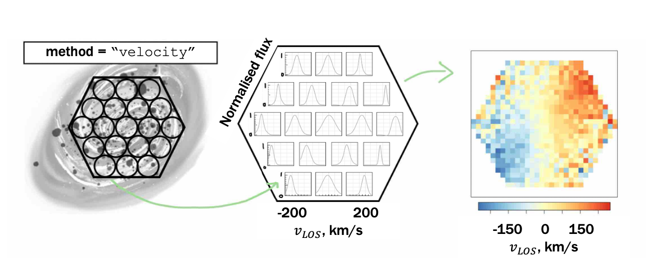
observation is the summary of the code. It contains information about how the observation has been constructed, such as the telescope parameters, the simulation parameters, the code version and run date. The full list output contains 34 different descriptors. These can be browsed above.

raw_images is a list with 7 elements that contain summary images of the observed simulation. The raw outputs contain the observations without observational parameters applied (such as the seeing conditions or line-spread-function).

# making a mask from the aperture region information included within the output$observation
mask = matrix(data = cube$observation$aperture_region, nrow = 30, ncol = 30)
mask[mask == 0] = NA

# plotting the raw images using the plot_images() functions within SimSpin:
plot_flux(cube$raw_images$flux_image*mask, labN = 1, fig = c(0,0.42,0.3,1), 
                 titleshift = -7, units = "g-band Flux, CGS")

plot_velocity(cube$raw_images$velocity_image*mask, fig = c(0.29,0.71,0.3,1), 
                 new=T, labN = 1, titleshift = -6)

plot_dispersion(cube$raw_images$dispersion_image*mask, fig = c(0.58,1,0.3,1), 
                 new=T, labN = 3, titleshift = -6)

plot_age(cube$raw_images$age_image*mask, fig = c(0,0.42,0,0.7), 
                 new=T, labN = 3, titleshift = -7)

plot_metallicity(cube$raw_images$metallicity_image*mask, fig = c(0.29,0.71,0,0.7), 
                 new=T, labN = 3, titleshift = -7)

plot_particles(cube$raw_images$particle_image*mask, fig = c(0.58,1,0,0.7), 
                 new=T, labN = 3, titleshift = -7)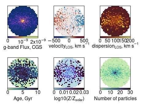

observed_images is a list with no elements in this case i.e. NULL.

To produce observational images from a spectral_cube, we need to run external software to fit templates to the spectrum in each pixel. This can be done using tools like pPXF. We demonstrate such an approach in the further examples “Fitting spectral cubes with pPXF”.

Note that, if method = "velocity", this element would contain 5 images generated by collapsing the resulting velocity_cube above.
variance_cube is also a list with no elements in this case (i.e. NULL), as the default telescope parameters list signal_to_noise as NA.

To produce a variance cube in this scenario, we need to specify a signal_to_noise value in the telescope function. The level of noise added to the spectral or velocity cube will then be recorded in the output list, for later use when fitting the kinematics using pPXF as described above.

Note that the units of these variance_cube lists have a factor of 1e40 contained, due to often very small flux values of order 1e-19. When taking the inverse square, these variance values become very large and standard precision may be insufficient. When written to FITS files, we divide the variance cube by 1e40 in order to avoid precision errors, but it is important to add these back in when fitting with pPXF.