Writing the data cube produced to a FITS file

Once you have build a mock observation, it is possible to save the output velocity or spectral cube, along with the associated images, to a FITS file that matches the common format for observational surveys using write_simspin_FITS.

The following code shows the default parameters used in the write_simspin_FITS function. This function is run in-line if, in build_datacube, you request a FITS file be produced (i.e write_fits = T). Else, it can be run seperately specifying the following elements:

write_simspin_FITS(output_file,              # where should the FITS file be written to?
                   simspin_datacube,                      # output from `build_datacube`
                   object_name, telescope_name, instrument_name,  # metadata information 
                   observer_name, input_simspin_file,                   
                   split_save=F,              # save cube and images to different files? 
                   mask=NA,                      # add a "mask" image to the output FITS
                   galaxy_centre = c(0,0,0)) # centre to give mock RA and Dec in outputs                   

Input parameters Output parameters See an example See the source code

Input Parameters

`output_file`	The path and file name to the location where the FITS file should be written. The code expects this path to end in “.fits” or “.FITS”.
`simspin_datacube`	The list output from the `build_datacube` function.
`object_name`	A string that described the name of the observed object.
`telescope_name`	A string that describes the name of the telescope used.
`instrument_name`	A string that describes the used instrument on that telescope.
`observer_name`	A string that describes the name of the observer.
`input_simspin_file`	A string describing the path to the original SimSpin file (i.e. the file output from make_simspin_file) such that the same FITS file can be made again in the future without the source code.
`split_save`	Boolean describing whether to split the output from `build_datacube` into multiple files. If TRUE, several FITS files will be saved with file names that reflect their content (i.e. “_spectral_cube.FITS”, “_velocity_image.FITS”,”_dispersion_images.FITS”, etc.). Default option is FALSE.
`telescope_name`	String used to describe the name of the telescope used for the observation in the FITS file header.
`observer_name`	String used to describe the name of the person who generated the observation in the FITS file header.
`split_save`	Only used when `write_fits = TRUE`. Should the output FITS be saved as one file with multiple HDUs to describe the output cube and observed images (`split_save = FALSE`)? Or should each cube/image be saved to a seperate file (`split_save = TRUE`)? In this case, the file name root will be taken from the state of `output_location` and descriptive names will automatically be appended to individual files (i.e. “_spectral_cube.FITS”, “_velocity_image.FITS”, etc.).
`mask`	(Optional) A binary array describing the masked regions of the cube/images, which will be saved to a seperate HDU.
`galaxy_centre`	(Optional) A numeric array (x,y,z) describing the centre of potential of the observed galaxy within it’s simulation. This infromation will be used in combination with the specified `Pointing` from `observing_strategy` to compute the RA and Dec within the HEADER information.

Output Parameters

The output of write_simspin_FITS is a FITS file that is written to the specified output_file location.

An example of how to extract the necessary information from the saved FITS can be found here.

The file will always contain at least two HDU elements, but a maximum of 17, though the contents of this file will change dependent on the mode in which the observation has been constructed and the input parameters specified above.

A summary of the maximum number of HDU extensions is shown below. This would be the result produced when a build_datacube observation has been run in method="velocity" mode, with a positive signal_to_noise value described within the telescope function and the FITS file has been written with split_save = F.

EXT (HDU)	Name	Description
1		Header containing general information relating to the individual galaxy observed, the code version run, and placeholder values to maintain typical FITS layout. i.e. the metadata for a given observation.
2	DATA	The kinematic cube with axes x, y, v_los. Each z-axis bin corresponds to a given LOS velocity, given by the axis labels. Values within each bin correspond to the amount of r-band flux at a given x-y projected location.
3	OB_TABLE	A table that contains all of the SimSpin run information such that a specific data cube can be recreated. Contains three columns (Name, Value, Units).
4	OB_FLUX	An image of the observed flux within the r-band in CGS units.
5	OB_VEL	An image of the observed line-of-sight (LOS) velocity in units of km/s.
6	OB_DISP	An image of the observed LOS velocity dispersion in units of km/s.
7	OB_H3	An image of the observed LOSVD higher order kinematic parameter, h3.
8	OB_H4	An image of the observed LOSVD higher order kinematic parameter, h4.
9	RESIDUAL	An image of the residual between the fitted LOSVD and observed distribution.
10	RAW_FLUX	An image of the raw particle flux in CGS in a given band specified by `filter` in the `telescope` function.
11	RAW_MASS	An image of the raw mass of particles per pixel in units of Msol.
12	RAW_VEL	An image of the raw particle LOS velocities in units of km/s.
13	RAW_DISP	An image of the raw particle LOS velocity dispersions in units of km/s.
14	RAW_AGE	An image of the raw particle stellar ages in units of Gyr.
15	RAW_Z	An image of the raw particle metallicities in units of Z_sol.
16	NPART	An image of the raw number of particles per pixel.
17	STAT	A 3D numeric array containing the variance cube for the observation.

Example

In order to save an observation to a file, we first need to produce an observation List to the environment. Let’s make a simple run of build_datacube using the SimSpin defaults:

# Using an example file from the package to build a SimSpin file:
simulation_data = system.file("extdata", "SimSpin_example_Gadget", 
                              package = "SimSpin")
                              
simspin_file    = make_simspin_file(filename = simulation_data, 
                                    disk_age = 5, # ages are assigned in Gyr
                                    bulge_age = 10, 
                                    disk_Z = 0.024, # metallicities are wrt solar 
                                    bulge_Z = 0.001,
                                    template = "BC03lr", # SSP template used
                                    write_to_file = FALSE) 

# Building a mock observation with default specifications for the telescope and observing strategy:
gadget_cube = build_datacube(simspin_file       = simspin_file, 
                             telescope          = telescope(signal_to_noise = 30),
                             observing_strategy = observing_strategy(),
                             method             = "velocity",
                             write_fits         = F)

# Running code to save the output observation to FITS:
write_simspin_FITS(simspin_datacube   = gadget_cube,        # build_datacube() output
                   output_file        = "gadget_cube.FITS", # filename of output file
                   input_simspin_file = simulation_data,    # filename of input sim     
                   object_name        = "GalaxyID_unknown", # name of observed object
                   telescope_name     = "Telescope",        # name of telescope
                   instrument_name    = "IFU",              # name of instrument 
                   observer_name      = "Anonymous")        # name of the observer

The output of running this code will be a FITS file written at the location specified by output_file. To explore this file within your R session, we suggest using the package Rfits, which can be downloaded here. We use the Rfits_info function to examine the structure of the file that has been written:

library("Rfits")
fits_summary = Rfits_info(filename = "gadget_cube.FITS")
fits_summary$summary

# [1] "SIMPLE  =                    T / file does conform to FITS standard"
# [2] "XTENSION= 'IMAGE   '           / IMAGE extension"                   
# [3] "XTENSION= 'BINTABLE'           / binary table extension"            
# [4] "XTENSION= 'IMAGE   '           / IMAGE extension"                   
# [5] "XTENSION= 'IMAGE   '           / IMAGE extension"                   
# [6] "XTENSION= 'IMAGE   '           / IMAGE extension"                   
# [7] "XTENSION= 'IMAGE   '           / IMAGE extension"                   
# [8] "XTENSION= 'IMAGE   '           / IMAGE extension"                   
# [9] "XTENSION= 'IMAGE   '           / IMAGE extension"                   
#[10] "XTENSION= 'IMAGE   '           / IMAGE extension"                   
#[11] "XTENSION= 'IMAGE   '           / IMAGE extension"                   
#[12] "XTENSION= 'IMAGE   '           / IMAGE extension"                   
#[13] "XTENSION= 'IMAGE   '           / IMAGE extension"                   
#[14] "XTENSION= 'IMAGE   '           / IMAGE extension"  
#[15] "XTENSION= 'IMAGE   '           / IMAGE extension"                   
#[16] "XTENSION= 'IMAGE   '           / IMAGE extension" 
#[17] "XTENSION= 'IMAGE   '           / IMAGE extension"                   

Here, we can clearly see that the file contains the sixteen HDU described in the table above: a header table, a binary table and a number of image extensions. The exact number of HDU can vary depending on the type of observation made by build_datacube. In all cases, HDU ext = 1 will always be the header information, HDU ext = 2 will always be the data cube produced and HDU ext = 3 will be a binary table containing the observation summary table used to produce the observation. In this case, for a velocity data cube there are a series of raw_images output into subsequent HDUs, followed by a number of observed_images.

By reading in the full file, we can see the names and sizes of these HDU below:

cube = Rfits_read_all("gadget_cube.FITS")
summary(cube)
#          Length Class        Mode
#              9  Rfits_header list
# DATA     58500  Rfits_cube   list
# OB_TABLE     3  Rfits_table  list
# OBS_FLUX   900  Rfits_image  list
# OBS_VEL    900  Rfits_image  list
# OBS_DISP   900  Rfits_image  list
# OBS_H3     900  Rfits_image  list
# OBS_H4     900  Rfits_image  list
# RESIDUAL   900  Rfits_image  list
# RAW_FLUX   900  Rfits_image  list
# RAW_MASS   900  Rfits_image  list
# RAW_VEL    900  Rfits_image  list
# RAW_DISP   900  Rfits_image  list
# RAW_AGE    900  Rfits_image  list
# RAW_Z      900  Rfits_image  list
# NPART      900  Rfits_image  list
# STAT     58500  Rfits_cube   list

This list would NOT include the observed images if the build_datacube method was “spectral”. In order to produce observational images, we need to use a tool like pPXF as demonstrated in the example “Fitting spectra with pPXF”.

Each element of the file can be accessed through their HDU name, for example:

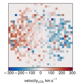
plot_velocity(cube$OBS_VEL$imDat) 
# where the "imDat" frame contains the image, with additional descriptors 
#  for each image included against that image as shown below

names(cube$OBS_VEL)
# [1] "imDat"       "keyvalues"   "keycomments" "keynames"    "header"      "hdr"         "raw"         "comment"    
# [9] "history"     "nkey"        "filename"    "ext"         "extname"     "WCSref"     

This is but a limited example to demonstrate how to save the output to a FITS file and then interact with the saved data. For more information about how to interact with these FITS files, please check out the example, “Working with FITS”.

At this stage, a mock observation may be processed like any other IFU observation, with half-light radii, Sersic indices and kinematic parameters measured. This is explored in a further example, “Using your mock observations”.

Beyond these examples, that is the end of the documentation for SimSpin functions. If you have missed any of the previous steps, please go back to the Documentation contents to browse other functions in the code. Else, enjoy mocking the Universe!