A walkthrough SimSpin’s functions
Here, we demonstrate how to create your first mock observation. At each step, we take you through the simplest routine using the default parameters for each function.
There are four steps to build your first SimSpin mock data cube:
- Making the input file
- Defining the observation properties
- Generating the observation
- Writing the output to FITS
We take you through each of these steps in the simplest form below. More extensive examples can be found in Examples.
Making the input file
The main input for SimSpin is a galaxy simulation. This may be either an isolated galaxy model (N-body or hydro-dynamical) or a region cut out from a cosmological simulation.
We define groups of particles or cells in each simulation according to the convention defined by Gadget (Springel, 2005):
PartType0- gas,PartType1- dark matter,PartType2- N-body disk,PartType3- N-body bulge,PartType4- stars,PartType5- boundary/black holes.
This information can be structured in an HDF5 file, with groups containing each of these particle types. Alternatively, SimSpin can also process Gadget binary files (SnapFormat type 1).
If you have any issues with your input simulation file, check out this page to check your input file structure.
We begin by running the make_simspin_file function. This will organise the provided data into a consistent format for SimSpin processing and assign SEDs to stellar particles given their individual ages and metallicities.
As this is the most time consuming process of the data-cube construction, we want to only do this once. However, a single SimSpin file can be usede multiple times for a variety of different observing strategies and telescope set ups. The variety of options available for this process is defined in the documentation here.
For this basic usage example, we will use the default parameters and one of the simple simulations included in the package:
simulation_data = system.file("extdata", "SimSpin_example_Gadget",
                              package = "SimSpin")

simspin_file    = make_simspin_file(filename = simulation_data,
                                    disk_age = 5, # ages are assigned in Gyr
                                    bulge_age = 10,
                                    disk_Z = 0.024, # metallicities are wrt solar
                                    bulge_Z = 0.001,
                                    template = "BC03lr", # SSP template used
                                    write_to_file = FALSE)
The output of this function will be a list that can either be written to an Rdata file or written to an environment variable within your R session. In the case above, we assign the output to the environment variable simspin_data.
Despite accepting a variety of different simulation inputs, the output of the make_simspin_file function will always be the same. The format will be a list containing 4 elements:
typeof(simspin_file)
# [1] "list"

summary(simspin_file)
#                    Length Class      Mode
# header                8   -none-     list
# star_part            12   data.frame list
# gas_part              0   -none-     NULL
# spectral_weights      2   -none-     list
While the length of each element may change depending on the input simulation type or observation properties requested, the element structure of the output will remain consistent.
In this case, because the input file is an N-body model containing both bulge and disk particles, the resulting element spectral_weights is a list with 2 entries (with one spectra assigned for the bulge particles and the second to the disk particles). For a hydrodynamical model, the spectral_weights element may have many more entries due to the broader variety in stellar ages and metallicities, but will remain an element of mode list.
Once a file has been produced for a single simulated galaxy, the same file can be used to produce any number of different observations.
Bear in mind that the resolution and wavelength range of the spectral templates used to generate the file need to overlap with the resolution and wavelength range of the observing telescope. You can check these parameters for a given template here. A WARNING will be issued by the code if these do not match.
Defining the observation properties
SimSpin acts as a virtual telescope. You can choose to observe your galaxy model in a variety of different ways with any integral field unit (IFU) instrument. This requires you to set two distinct groups of properties - the properties of the instrument used to take the observation i.e. the telescope, and the properties of the object under scrutiny i.e. the observing_strategy.
telescope
This class describes the properties of the instrument used for the observation. Several current instruments are included within the class (named by either the telescope or the survey that used them i.e. SAMI, MaNGA, CALIFA and MUSE) but you can also define your own instrument by specifying the type = 'IFU'.
An example of a user defined instrument is shown below, with the default parameters specified:
ifu = telescope(type = "IFU", # other options include pre-defined instruments
                fov = 15, # field-of-view in arcsec
                aperture_shape = "circular", # shape of fov
                wave_range = c(3700,5700), # given in angstroms
                wave_centre = 4700, # central wavelength given in angstroms
                wave_res = 1.04, # wavelength resolution in angstroms
                spatial_res = 0.5, # size of spatial pixels in arcsec
                filter = "r", # filter for calc of particle luminosity
                lsf_fwhm = 2.65, # full-width half-max of line-spread-function
                signal_to_noise = 10) # s/n ratio per angstrom
This will return a list that contains 11 elements. Here we have precomputed properties that will be necessary for further computation steps. The units of each returned element have been added in the final column.
typeof(ifu)
# [1] "list"

summary(ifu)
#                 Length Class      Mode        # Units
# type            1      -none-     character   # describes the telescope
# fov             1      -none-     numeric     # field of view diameter arcsec
# aperture_shape  1      -none-     character   # shape of fov
# wave_range      2      -none-     numeric     # angstrom
# wave_centre     1      -none-     numeric     # angstrom
# wave_res        1      -none-     numeric     # angstrom
# spatial_res     1      -none-     numeric     # arcsec per pixel
# filter_name     1      -none-     character   # name of chosen filter
# filter          2      data.table list        # filter wavelengths and response
# lsf_fwhm        1      -none-     numeric     # angstrom
# signal_to_noise 1      -none-     numeric     # signal-to-noise ratio
# sbin            1      -none-     numeric     # number of spatial bins across fov
observing_strategy
We describe the conditions of the object begin observed using this function. For example, the level of atmospheric blurring can be modified, the angle from which the object is observed can be changed and the distance at which the galaxy is projected can be adjusted.
An example with the default parameters specified is shown here:
strategy = observing_strategy(dist_z = 0.05, # redshift distance the galaxy is placed
                              inc_deg = 70, # projection (0 - face-on, 90 - edge-on)
                              twist_deg = 0, # angle of observation (longitude)
                              pointing_kpc = c(0,0), # pointing of the centre of the telescope
                              blur = F, # whether seeing conditions are included
                              fwhm = 2, # the fwhm of the blurring kernel in arcsec
                              psf = "Gaussian") # the shape of the blurring kernel
This will return a list that contains 5 elements. If blur = T, an additional two elements will be included to describe the point-spread-function shape and size. Similar to the previous output, this class just stores precomputed properties relevant to the observed object that will be necessary in further processing steps. The units of each returned element are listed in the final column.
typeof(strategy)
# [1] "list"

summary(strategy)
#           Length Class    Mode    # Units
# distance  1      Distance S4      # either redshift distance (z), physical (Mpc) or angular (kpc per arcsec)
# inc_deg   1      -none-   numeric # degrees
# twist_deg 1      -none-   numeric # degrees
# pointing  1      Pointing S4      # either physical (kpc) or angular (deg)
# blur      1      -none-   logical # FWHM specified in arcseconds
With these properties specified, we have fully described the parameters necessary to construct the observation.
Generating the observation
Once the particulars of the observation have been defined, we can go ahead and make the observation. This means feeding our prepared parameters into the build_datacube function.
An example is shown below.
gadget_cube = build_datacube(simspin_file       = simspin_file,
                             telescope          = ifu,
                             observing_strategy = strategy,
                             method             = "spectral",
                             write_fits         = F)
We choose not to write the output directly to file (write_fits = F) and output to a variable called gadget_cube instead.
The returned variable will always be a list containing 4 elements:
- the first always being the data cube,
- followed by the observation summary,
- raw simulation images and
- mock observation images generated from collapsing the data cube.
> typeof(gadget_cube)
# [1] "list"
> summary(gadget_cube)
#                 Length  Class  Mode
# spectral_cube   1731600 -none- numeric
# observation          36 -none- list
# raw_images            7 -none- list
# observed_images       0 -none- NULL
For a detailed description of each of these outputs, see the output parameters in build_datacube.
The overall format of this output will be consistent regardless of the inputs of build_datacube. However, the names of individual elements change to reflect the variety in the requested properties specified by telescope and observing_strategy. The method of observation will also modify the length of each element.
- For example,
method = 'spectral'will return a variablespectral_cubeas its first element; specifying insteadmethod = 'velocity'will return avelocity_cube. - The
observed_imageselement will beNULLwhen a cube is built withmethod = 'spectral', as observational images must be generated using external software such as pPXF.
Writing the output to FITS
Using the write_simspin_FITS function, the new observation can be written to a file that can be shared or re-analysed using observational pipelines. SimSpin can write such a FITS file using the variable produced by build_datacube.
A few further descriptive details are suggested as input for users of the file later on, but the function defaults to sensible suggestions.
An example is shown in the code below.
write_simspin_FITS(simspin_datacube   = gadget_cube,        # build_datacube() output
                   output_file        = "gadget_cube.FITS", # filename of output file
                   input_simspin_file = simulation_data,    # filename of input sim
                   object_name        = "GalaxyID_unknown", # name of observed object
                   telescope_name     = "Telescope",        # name of telescope
                   instrument_name    = "IFU",              # name of instrument
                   observer_name      = "Anonymous")        # name of the observer
The output of running this code will be a FITS file written at the location specified by output_file. To explore this file within your R session, we suggest using the HeaderExt branch of the package Rfits, which can be downloaded here. We use the Rfits_info function to examine the structure of the file that has been written:
library("Rfits")
fits_summary = Rfits_info(filename = "gadget_cube.FITS")
fits_summary$summary

# [1] "SIMPLE  =                    T / file does conform to FITS standard"
# [2] "XTENSION= 'IMAGE   '           / IMAGE extension"
# [3] "XTENSION= 'BINTABLE'           / binary table extension"
# [4] "XTENSION= 'IMAGE   '           / IMAGE extension"
# [5] "XTENSION= 'IMAGE   '           / IMAGE extension"
# [6] "XTENSION= 'IMAGE   '           / IMAGE extension"
# [7] "XTENSION= 'IMAGE   '           / IMAGE extension"
# [8] "XTENSION= 'IMAGE   '           / IMAGE extension"
# [9] "XTENSION= 'IMAGE   '           / IMAGE extension"
Here, we can clearly see that the file contains six HDU: a header table and a number of images. The exact number of HDU can vary depending on the type of observation made by build_datacube. In all cases, HDU ext = 1 will always be the header information and HDU ext = 2 will always be the data cube produced. In this case, for a spectral data cube there are a series of raw_images output into subsequent HDUs. In the case of a velocity data cube, we would also see several observed_images included in the output.
The first HDU (ext = 1) is a header element describes the properties of the observation. This acts as a record for reproducing that identical observation again in the future. Information that is recorded in the header is listed below. These are consistent across all FITS files written using this function, regardless of variety in build_datacube options.
head = Rfits_read_header("gadget_cube.FITS")
head$header
# [1] "SIMPLE  =                    T / file does conform to FITS standard"
# [2] "BITPIX  =                    8 / number of bits per data pixel"
# [3] "NAXIS   =                    0 / number of data axes"
# [4] "EXTEND  =                    T / FITS dataset may contain extensions"
# [5] "COMMENT   FITS (Flexible Image Transport System) format is defined in 'Astronomy"
# [6] "COMMENT   and Astrophysics', volume 376, page 359; bibcode: 2001A&A...376..359H"
# [7] "ORIGIN  = 'SimSpin_v2.4.5.5'   / Mock observation"
# [8] "TELESCOP= 'Telescope'          / Telescope name"
# [9] "INSTRUME= 'IFU     '           / Instrument used"
#[10] "RA      =                    0 / [deg] 11:41:21.1 RA (J2000) pointing"
#[11] "DEC     =                    0 / [deg] -01:34:59.0 DEC (J2000) pointing"
#[12] "EQINOX  =                 2000 / Standard FK5"
#[13] "RADECSYS= 'FK5     '           / Coordinate system"
#[14] "EXPTIME =                 1320 / Integration time"
#[15] "MJD-OBS =             58906.11 / Obs start"
#[16] "DATE-OBS= '2023-03-27 15:48:22' / Observing date"
#[17] "UTC     =                 9654 / [s] 02:40:54.000 UTC"
#[18] "LST     =             30295.18 / [s] 08:24:55.178 LST"
#[19] "PI-COI  = 'UNKNOWN '           / PI-COI name."
#[20] "OBSERVER= 'Anonymous'          / Name of observer."
#[21] "REDSHIFT=                 0.05 / Observed redshift."
#[22] "PIPEFILE= 'gadget_cube.FITS'   / Filename of data product"
#[23] "BUNIT   = 'erg/s/cm**2'        / Angstrom"
#[24] "ARCFILE = '/home/username/R/x86_64-pc-linux-gnu-library/4.2/SimSpin/extdata/SimS'"
#[25] "DATAMD5 = '4aece79473a5c88f6533382655e948bf' / MD5 checksum"
#[26] "OBJECT  = 'GalaxyID_unknown'   / Original target."
Observing details such as the name of the person who ran the file, the name of the object and the redshift at which is was observed are all included in this header. Importantly, we also record the name and location of the SimSpin file from which this observation was made (denoted as ARCFILE), enabling files to be reproduced in the future. Similarly, the SimSpin version number is recorded within the ORIGIN element with the added description that this is a mock observation. Admittedly, several aspects to this header have to be invented as they do not have any physical meaning for mock observations (RA and DEC, for example), but are required for consistency with their observational counterparts.
Finally, we can go about reading in and working with the data cube itself. Each HDU comes along with its own header to describe the properties of the image contained i.e. the units and dimensions of the pixels. These details can be used to examine and process the data.
cube = Rfits_read_all("gadget_cube.FITS")
summary(cube)
#          Length  Class        Mode
#                9 Rfits_header list
# DATA     1731600 Rfits_cube   list
# OB_TABLE       3 Rfits_table  list
# RAW_FLUX     900 Rfits_image  list
# RAW_VEL      900 Rfits_image  list
# RAW_DISP     900 Rfits_image  list
# RAW_AGE      900 Rfits_image  list
# RAW_Z        900 Rfits_image  list
# NPART        900 Rfits_image  list
Having read in all HDU from the FITS file, we can then visualise elements from the saved spectral cube cube$DATA using the wavelength information included in the observation meta-data cube$OB_TABLE:
cube$OB_TABLE
#               Name               Value    Units
# 1:        ang_size             1.00032    num: scale at given distance in kpc/arcsec
# 2:  aperture_shape            circular    str: shape of aperture
# 3:   aperture_size             15.0048    num: field of view diameter width in kpc
# 4:            date 2023-03-27 15:48:22    str: date and time of mock observation
# 5:             fov                  15    num: field of view diameter in arcsec
# 6:          filter              r_SDSS    str: filter name
# 7:         inc_deg                  70    num: projected inclination of object in degrees about the horizontal axis
# 8:         inc_rad             1.22173    num: projected inclination of object in radians about the horizontal axis
# 9:       twist_deg                   0    num: projected inclination of object in degrees about the vertical axis
#10:       twist_rad                   0    num: projected inclination of object in radians about the vertical axis
#11:        lsf_fwhm                2.65    num: line-spread function of telescope given as full-width half-maximum in Angstrom
#12:        lum_dist              227.48    num: distance to object in Mpc
#13:       mass_flag               FALSE    bool: kinematics are mass weighted if TRUE
#14:          method            spectral    str: name of observing method employed
#15:          origin    SimSpin_v2.4.5.5    str: version of SimSpin used for observing
#16:    pointing_kpc                 0,0    num: x-y position of field of view centre relative to object centre in units of kpc
#17:    pointing_deg                 0,0    num: x-y position of field of view centre relative to object centre in units of degrees
#18:        psf_fwhm                   0    num: the full-width half-maximum of the point spread function kernel in arcsec
#19:            sbin                  30    num: the number of spatial pixels across the diameter of the field of view
#20:        sbin_seq      -7.5024,7.5024    num: the min and max spatial bin centres in kpc
#21:       sbin_size             0.50016    num: the size of each pixel in kpc
#22:     spatial_res                 0.5    num: the size of each pixel in arcsec
#23: signal_to_noise                  10    num: the signal-to-noise ratio for observed spectrum
#24:        wave_bin                1924    num: the number of wavelength bins for a given telescope
#25:     wave_centre                4700    num: the central wavelength for a given telescope in Angstrom
#26:        wave_res                1.04    num: the width of each wavelength bin in Angstrom
#27:        wave_seq        3700,5699.92    num: the min and max wavelength bin centres in Angstrom
#28:      wave_edges     3699.48,5700.44    num: the wavelength bin edges in Angstrom
#29:       vbin_size             66.3371    num: the size of each velocity bin in km/s
#30:      vbin_error             71.7812    num: the velocity uncertainty given the telescope LSF in km/s
#31:               z                0.05    num: the redshift distance of the object observed
#32:        LSF_conv               FALSE    bool: has line spread function convolution been applied?
#               Name               Value    Units
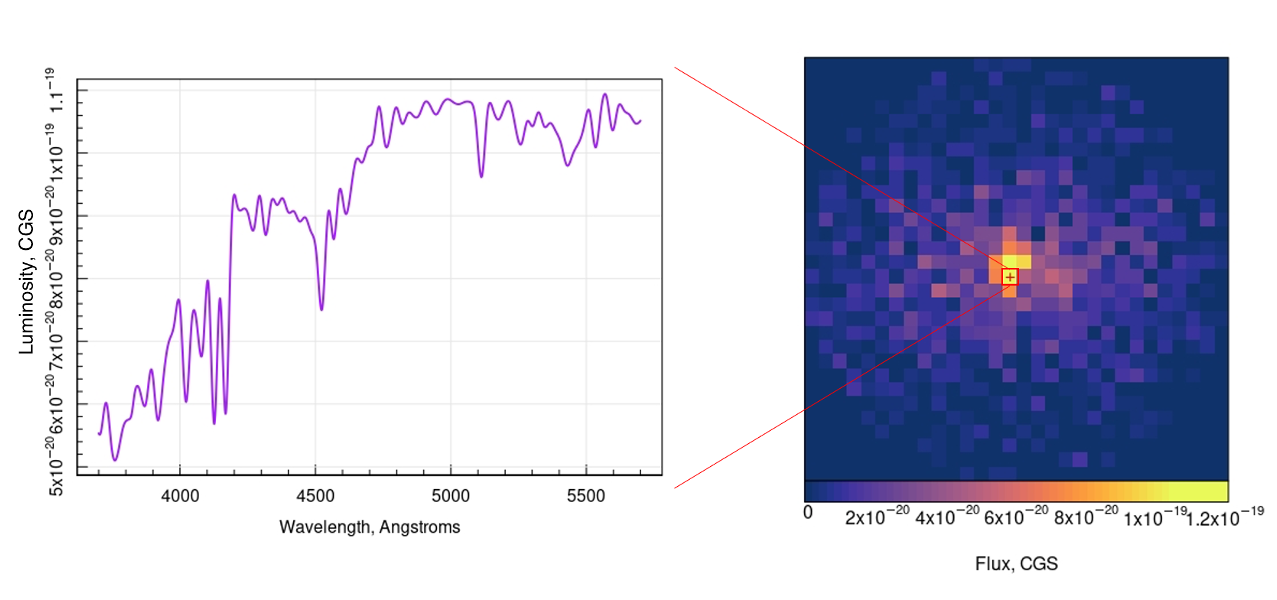
Using the values in elements [26] and [27], we can define the wavelength range for each spectrum in the cube and plot a given output with the appropriate labels.
wavelength_range = as.numeric(stringr::str_split(string = cube$OB_TABLE$Value[27], pattern = ",")[[1]])
wavelength_seq   = seq(wavelength_range[1], wavelength_range[2], by = as.numeric(cube$OB_TABLE$Value[26]))

# examining the central spaxel of the output spectral cube:
magicaxis::magplot(wavelength_seq, cube$DATA[["imDat"]][15,15,], type="l", col = "purple", lwd =2, xlab = "Wavelength, Angstroms", ylab = "Luminosity, CGS")

# plotting the flux image saved to the cube:
plot_flux(cube$RAW_FLUX$imDat)
points(x = 14.5, y = 14.5, pch="+", col="red")
This demonstrates a basic way to interact with the data that has been saved to a FITS file. Similar methodology can be used to examine both the 3-dimensional data cubes and the 2-dimensional images contained within sequential HDUs. For further examples working with FITS files, check out “Working with FITS files from SimSpin” in the examples on the left.
These steps can be used to generate a mock observation of a simulated galaxy. In this Basic Usage section, we have run the simplest recipe using the inbuilt defaults of each function. In the next section, we go into details of additional functionality that may be relevant for your work.