Using your mock observation (now that it’s built!)
Now you’ve got your mock IFU observation of a simulated galaxy, what can you do with it? The aim is to produce a FITS file that can be used in the same way as true IFU observations of real galaxies. So, the hope is that you can process these observations with your favourite analysis codes already in use.
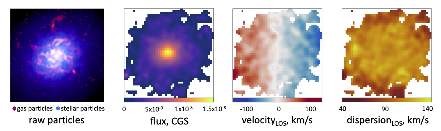
In these examples, we will be using this mock observation. We have selected a disk galaxy from the EAGLE simulation from the z=0 box of RefL0100N1504 (GalaxyID 16653664). We’ve built a MUSE observation of this system in velocity mode such that we can examine the kinematics of the system without first having to fit these using pPXF.
You can download your own copy of this observation file here.
Fitting isophotes
We will be using R-packages, such as Profit and Profound, to fit isophotal ellipses to the flux map image. Using these isophotes, we can measure the light profile of our system and define the half-light radius in an equivalent manner to observations. Within this aperture, we can then measure the kinematics of the system.
If Python or Julia is your preference, SimSpin can produce FITS files for processing with your favourite analysis codes. For example, check out the pPXF walk-through here.
In this example, we will be using a number of functions that are not within the SimSpin package. Each function is highlighted in code snippets below.
# Loading the following packages for our processing requirements:
library(SimSpin)
library(magicaxis)
library(ProFound)
library(ProFit)
library(Rfits)
All of these packages should be installed when the installation of SimSpin is run, as explained here. If any are missing, you should find them available through CRAN (or, in the case of ProFit and ProFound, on GitHub at each link respectfully).
Having produces FITS files using build_datacube, we read in the images using the Rfits package as shown below. We define our segmentation map in order to specify the region to which isophotal ellipses should be fit using the 25th percentile flux limit, as shown in the definition of the mask parameter. This produces the white edge to the region in the images above.
dir = "/c39d4a8a-2ef9-4a12-b353-f984fd2def7a_bundle/"

flux       = Rfits::Rfits_read_all(paste0(dir,
             "EAGLE_snap28_50kpc_with_galaxyID_16653664_BC03lr
             _inc30deg_seeing0.6fwhm_obs_flux_image.FITS"))$OBS_FLUX$imDat

velocity   = Rfits::Rfits_read_all(paste0(dir,
             "EAGLE_snap28_50kpc_with_galaxyID_16653664_BC03lr
             _inc30deg_seeing0.6fwhm_obs_velocity_image.FITS"))$OBS_VEL$imDat

dispersion = Rfits::Rfits_read_all(paste0(dir,
             "EAGLE_snap28_50kpc_with_galaxyID_16653664_BC03lr
             _inc30deg_seeing0.6fwhm_obs_dispersion_image.FITS"))$OBS_DISP$imDat

mask = flux
mask[flux < quantile(flux, c(0.25))] = 0
mask[!is.na(mask)] = 1 # initial segmentation map
We then use the flux image and mask produced to fit isophotal ellipses using ProFound. We select the number of ellipses we would like to fit (in this case, 16) and provide the pixel scale (0.2 “/pixel for a MUSE observation) such that the output radial measurements are output in units of arcseconds.
ellipse_data = ProFound::profoundGetEllipses(image = flux,
                                             pixscale = 0.2, # "/pixel
                                             segim = mask,
                                             levels = 16,
                                             plot = T)
Using these fitted isophotes, we can then define things like the half-light radius and ellipticity. These are taken as the mean isophote containing 50% of the flux as shown in the code snippen below.
It is worth noting here that, with simulations, we have full knowledge of the total mass of the galaxy in question. In cases where the full galaxy is not contained within the mock image, these isophotes can be scaled appropriately to reflect the true half-light radius position.
flux_frac = ellipse_data$ellipses$fluxfrac
hm_id = which(abs(flux_frac-0.5) == min(abs(flux_frac-0.5)))
um_id = which(abs(flux_frac-0.6) == min(abs(flux_frac-0.6)))
lm_id = which(abs(flux_frac-0.4) == min(abs(flux_frac-0.4)))
isops = lm_id:um_id

ellipticity = mean(1 - ellipse_data$ellipses$axrat[isops])
ellipticity_error = sd(1 - ellipse_data$ellipses$axrat[isops])
primary_axis = mean(ellipse_data$ellipses$ang[isops])
primary_axis_error = sd(ellipse_data$ellipses$ang[isops])
major_axis_a =  mean(ellipse_data$ellipses$radhi[isops]) # size in "
minor_axis_b =  mean(ellipse_data$ellipses$radlo[isops]) # size in "
| ellipticity, ε | Δ ε | Principle Axis, degrees | Δ PA, degrees | a, “ | b, “ |
|---|---|---|---|---|---|
| 0.22 | 0.06 | 130 | 23 | 3.14 | 2.47 |
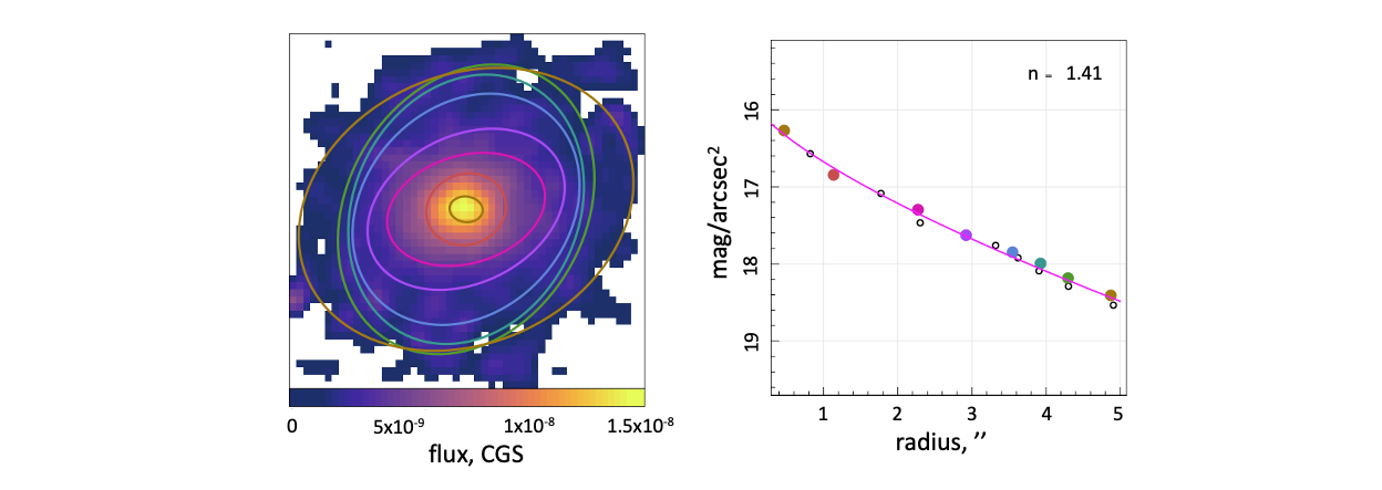
We show these chosen ellipses on the original flux image and plot the surface brightness as a function of radius beside this. Using the Sersic profile defined within the ProFit package, we can fit this surface brightness profile to determine the Sersic index of the galaxy in this image.
onecomponent=function(par=c(20, 3, 3), rad, SB, pixscale=1){
  bulge=ProFit::profitRadialSersic(rad, mag=par[1], re=par[2], nser=par[3])
  total=ProFound::profoundFlux2SB(bulge, pixscale=pixscale)
  return=sum((total-SB)^2)
} # define a 1D fitting function to the surface brightness profile

model_fit = optim(onecomponent, par=c(-25, 5, 5),
                  rad=ellipse_data$ellipses$radhi, SB=ellipse_data$ellipses$SB, pixscale=0.2,
                  method='BFGS')$par
rlocs=seq(0,5,by=0.1)
galaxy=ProFit::profitRadialSersic(rlocs, mag=model_fit[1], re=model_fit[2], nser=model_fit[3])
To plot these summary images, we introduce another two packages (which can both be installed from CRAN using install.packages("cmocean") and install.packages("plotrix") respectfully).
library(cmoean)
library(plotrix)

plot_flux(flux_image = flux)
plotrix::draw.ellipse(ellipse_data$ellipses$xcen[seq(1,16,by=2)],
                      ellipse_data$ellipses$ycen[seq(1,16,by=2)],
                      ellipse_data$ellipses$radhi[seq(1,16,by=2)]/0.2,
                      ellipse_data$ellipses$radlo[seq(1,16,by=2)]/0.2,
                      (ellipse_data$ellipses$ang[seq(1,16,by=2)]-90),
                      border = cmocean::cmocean("phase")(8), density = NULL, lwd=3)

magplot(ellipse_data$ellipses$radhi, ellipse_data$ellipses$SB, pch = 1,
        ylim=c(max(ellipse_data$ellipses$SB, na.rm = TRUE)+1,min(ellipse_data$ellipses$SB, na.rm = TRUE)-1),
        type='p', xlab=' radius / "', ylab=expression('mag / arcsec'^2), lwd = 2)
points(ellipse_data$ellipses$radhi[seq(1,16,by=2)], ellipse_data$ellipses$SB[seq(1,16,by=2)],
       col = cmocean::cmocean("phase")(8), pch = 16, cex=2)
lines(rlocs, ProFound::profoundFlux2SB(galaxy, pixscale=0.2), col='magenta', lwd=2)
legend("topright", inset = c(0.05,0.05), legend=parse(text=sprintf('n == %f', model_fit[3])), text.col = "black", bty="n")
Measuring kinematics within the effective radius
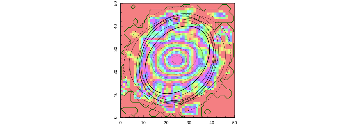
Now that we have fitted the half-light ellipse, we can go about measuring the kinematics within this region. We do this simply by defining the isophotal ellipse as a mask and only using suitable spaxels within this region to compute things like the observable spin parameter, λR.
\[\lambda_R = \frac{\sum{F R V}}{\sum{F R\sqrt{V^2 + \sigma^2}}}\]In order to measure this parameter, we compute the elliptical radius, the line-of-sight velocity and dispersion per pixel within the effective isophotal ellipse and perform a light-weighted sum of each pixel.
# Next computing the kinematics within the 1Re ellipse:
.ellipse = function(a, b, x, y, ang_deg){
  ang_rad = (ang_deg+90) * (pi/180)
  r = ((x*cos(ang_rad) + y*sin(ang_rad))^2 /a^2) + ((x*sin(ang_rad) - y*cos(ang_rad))^2 / b^2)
  return(r)
}

# Defining the 1Re mask
kin_mask = array(data = NA, dim = dim(flux))
xcentre = ellipse_data$ellipses$xcen[8]
ycentre = ellipse_data$ellipses$ycen[8]
mask[xcentre, ycentre] = 1

# Semi-major axis in units of pixels
a = major_axis_a/0.2
# Semi-minor axis in units of pixels
b = minor_axis_b/0.2

for (x in 1:50){
  for (y in 1:50){
    xx = (x - xcentre)
    yy = (y - ycentre)
    rr = .ellipse(a = a, b = b, x = xx, y = yy, ang_deg = primary_axis)
    if (rr <= 1){
      kin_mask[x,y] = 1
    }
  }
}

# Computing the ellipsoidal radius at each pixel position
x = seq(1,50)
sbin = 50 # number of spaxels in each dimension
sbin_grid = list("x" = array(data = rep(x-xcentre, sbin), dim = c(sbin,sbin)),
                 "y" = array(data = rep(x-ycentre, each=sbin), dim = c(sbin,sbin)))
radius = .ellipse(a, b, sbin_grid$x, sbin_grid$y, primary_axis)

# Masking the original maps
masked_radius = radius*kin_mask
masked_flux = flux*kin_mask
masked_vel = velocity*kin_mask
masked_disp = velocity*kin_mask

plot_flux(masked_radius, units = "Radius, R eff")
plot_flux(masked_flux)
plot_velocity(masked_vel)
plot_dispersion(masked_disp)

With these parameters measured within the ellipse, we can then use these spaxels to compute the λR parameter, as in the code snippet below.
sum(masked_flux * abs(masked_vel) * masked_radius, na.rm = T) / sum(masked_flux * masked_radius * sqrt(masked_vel^2 + masked_disp^2), na.rm=T)

0.707
We find, within an effective radius, this system has a high spin parameter of λR = 0.7.
Several further measurements can be made using similar techniques. We conclude this example at this point, but encourage you to get in touch if you would be keen to see other analysis using SimSpin data products by raising an issue below: